Use Cases

Use Cases:

1. Denoising a picture

In this example, we denoise a noisy version of a picture using the total variation, bilateral, and wavelet denoising filters.

Total variation and bilateral algorithms typically produce “posterized” images with flat domains separated by sharp edges. It is possible to change the degree of posterization by controlling the tradeoff between denoising and faithfulness to the original image.

import matplotlib.pyplot as plt

from skimage.restoration import (
    denoise_tv_chambolle,
    denoise_bilateral,
    denoise_wavelet,
    estimate_sigma,
)
from skimage import data, img_as_float
from skimage.util import random_noise


original = img_as_float(data.chelsea()[100:250, 50:300])

sigma = 0.155
noisy = random_noise(original, var=sigma**2)

fig, ax = plt.subplots(nrows=2, ncols=4, figsize=(8, 5), sharex=True, sharey=True)

plt.gray()

# Estimate the average noise standard deviation across color channels.
sigma_est = estimate_sigma(noisy, channel_axis=-1, average_sigmas=True)
# Due to clipping in random_noise, the estimate will be a bit smaller than the
# specified sigma.
print(f'Estimated Gaussian noise standard deviation = {sigma_est}')

ax[0, 0].imshow(noisy)
ax[0, 0].axis('off')
ax[0, 0].set_title('Noisy')
ax[0, 1].imshow(denoise_tv_chambolle(noisy, weight=0.1, channel_axis=-1))
ax[0, 1].axis('off')
ax[0, 1].set_title('TV')
ax[0, 2].imshow(
    denoise_bilateral(noisy, sigma_color=0.05, sigma_spatial=15, channel_axis=-1)
)
ax[0, 2].axis('off')
ax[0, 2].set_title('Bilateral')
ax[0, 3].imshow(denoise_wavelet(noisy, channel_axis=-1, rescale_sigma=True))
ax[0, 3].axis('off')
ax[0, 3].set_title('Wavelet denoising')

ax[1, 1].imshow(denoise_tv_chambolle(noisy, weight=0.2, channel_axis=-1))
ax[1, 1].axis('off')
ax[1, 1].set_title('(more) TV')
ax[1, 2].imshow(
    denoise_bilateral(noisy, sigma_color=0.1, sigma_spatial=15, channel_axis=-1)
)
ax[1, 2].axis('off')
ax[1, 2].set_title('(more) Bilateral')
ax[1, 3].imshow(
    denoise_wavelet(noisy, channel_axis=-1, convert2ycbcr=True, rescale_sigma=True)
)
ax[1, 3].axis('off')
ax[1, 3].set_title('Wavelet denoising\nin YCbCr colorspace')
ax[1, 0].imshow(original)
ax[1, 0].axis('off')
ax[1, 0].set_title('Original')

fig.tight_layout()

plt.show()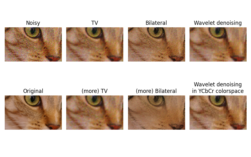

Output

2. Face detection using a cascade classifier

Face recognition is widely used in security, user authentication, and emotion detection. This computer vision example shows how to detect faces on an image using object detection framework based on machine learning.

from skimage import data
from skimage.feature import Cascade

import matplotlib.pyplot as plt
from matplotlib import patches

# Load the trained file from the module root.
trained_file = data.lbp_frontal_face_cascade_filename()

# Initialize the detector cascade.
detector = Cascade(trained_file)

img = data.astronaut()

detected = detector.detect_multi_scale(
    img=img, scale_factor=1.2, step_ratio=1, min_size=(60, 60), max_size=(123, 123)
)

fig, ax = plt.subplots()
ax.imshow(img, cmap='gray')

for patch in detected:
    ax.axes.add_patch(
        patches.Rectangle(
            (patch['c'], patch['r']),
            patch['width'],
            patch['height'],
            fill=False,
            color='r',
            linewidth=2,
        )
    )

plt.show()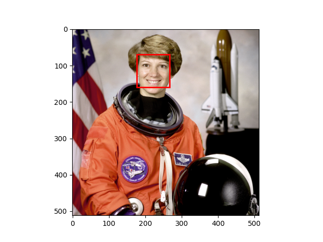

Output

3. Render text onto an image

Rendering text onto an image is a common technique used in various real-world applications.

import matplotlib.pyplot as plt
import numpy as np
from skimage import data

img = data.cat()

fig = plt.figure()
fig.figimage(img, resize=True)
fig.text(0, 0.99, "I am stefan's cat.", fontsize=32, va="top")
fig.canvas.draw()
annotated_img = np.asarray(fig.canvas.renderer.buffer_rgba())
plt.close(fig)

fig, ax = plt.subplots()
ax.imshow(annotated_img)
ax.set_axis_off()
ax.set_position([0, 0, 1, 1])
plt.show()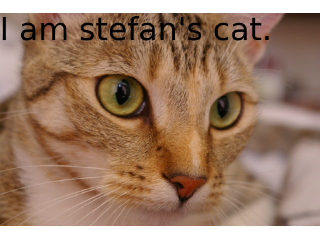

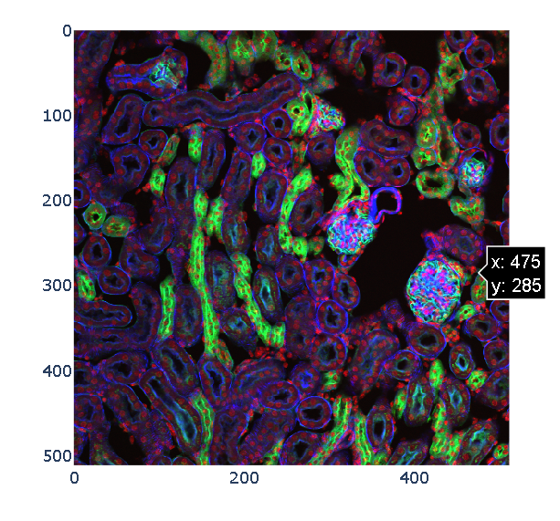
Output

4. Medical Image Processing

Example: Interact with 3D images (of kidney tissue)

1. Load image

This biomedical image is available through scikit-image’s data registry.

import matplotlib.pyplot as plt
import numpy as np

import plotly
import plotly.express as px
from skimage import data
data = data.kidney()

n_plane, n_row, n_col, n_chan = data.shape

Let us consider only a slice (2D plane) of the data for now. More specifically, let us consider the slice located halfway in the stack. The imshow function can display both grayscale and RGB(A) 2D images.

_, ax = plt.subplots()
_, ax = plt.subplots()
ax.imshow(data[n_plane // 2])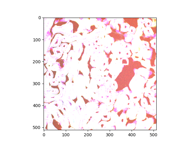

Output

We turn to Plotly’s implementation of the plotly.express.imshow() function, for it supports value ranges beyond (0.0, 1.0) for floats and (0, 255) for integers.

vmin, vmax = data.min(), data.max()
fig = px.imshow(data[n_plane // 2], zmax=vmax)
plotly.io.show(fig)

Output